Understanding the deepwater frontier
Stephen O’Connor, Sam Green, Alexander Edwards, Dean Thorpe, Phill Clegg and Eamonn Doyle, Ikon Science, explain de-risking deepwater drilling and exploration by applying simple geological rules from analogue situations.
A recent article published by Nelson et al. (2013) stated, firstly, that deepwater has become the predominant source of new oil and gas discoveries worldwide, accounting for more than 50% of all conventional new reserves of 170 billion boe.1 Secondly, six-year trend data (between 2007 and 2012) shows that average hydrocarbon discovery size is considerably larger offshore, especially so in the deepwater, where discovery sizes reached 230 million boe. This is about an order of magnitude larger than the onshore average new discovery size for the same period, which is approximately 20 million boe.
Indeed, the authors estimated that approximately 200 oil and gas companies participated in deepwater exploration drilling globally during this period, with 950 new-field wildcat wells drilled. However, drilling success rates averaged only 10 - 15% globally. This last comment is not particularly surprising as the deepwater environment has many inherent risks due to a general lack of well calibration such that there can be (a) an elevated risk of geological failure, i.e., no hydrocarbons present, as well as (b) a higher risk of well control problems during drilling as the uncertainty in the pre-drill pore pressure estimation is greater.
Surprisingly, however, there are companies, especially the small and medium independents, that have demonstrated high exploration efficiencies in terms of drilling success rates and reserves-additions per well.1 The key to their success has been attributed by the same authors to a clear exploration strategy that focuses on specific basins and play types. These companies make good use of analogues from proven plays and apply new geological concepts in older exploration areas. Targeting similar plays in new basins such as those in offshore Suriname and French Guiana as previously explored in West Africa, as well as targeting deeper stratigraphy in existing basins, e.g. Cretaceous (Campanian and Turonian) plays in West Africa. Figure 1 shows the main areas of current deepwater drilling.

Figure 1. Location map showing areas of deep- and ultra-deep water globally.9
The focus of this article is pore pressure, and discusses how one can use analogues to de-risk future well planning, i.e., what are the typical characteristics of deepwater systems and how do these influence the development of the pore pressure regime? The approach is a geologically-driven one and assumes the simple premise that the same rocks (and basin history) equates to the same pressure regime. The authors also stress how important real time data (data acquired during the drilling process) is/can be in terms of further reducing risk and uncertainty when drilling commences. There is a general assumption that all risk assessment is conducted pre-drill. Whereas in reality, assessing risk and uncertainty continues or should continue into the drilling phase where hard data received from the drill bit and the surrounding environment can be vital as a look-ahead warning. In addition to the well planning benefit, analysing analogue basins for pore pressure means that it might be possible to de-risk plays for mechanical top-seal failure (where the pore pressure in our prospect reservoir is deemed too high resulting in an elevated risk of seal failure).
Success and failure in the deepwater
In recent years there have been a series of success stories in the deepwater:1
- Mozambique and Tanzania, approximately 8 trillion ft3 of gas was reported discovered in Eocene and Paleocene stratigraphic plays.
- Another significant gas discovery of 5.7 trillion ft3 was made in a Lower Miocene play in Israel and Cypress (Levantine basin) e.g. Tamar and Leviathan.
- In Ghana, a significant oil and gas volume of almost 2 billion boe was made in a Turonian stratigraphic and Turonian stratigraphic-structural plays in the Cote d'Ivoire basin. The ‘Jubilee’ discovery in many ways was a real game-changer.
- Other new, significant deepwater plays were established off French Guiana, e.g. the Zaeydus discovery, as well as other regions including the Falkland Islands, Norway, Iran, Mexico and India.
However, there have also been a number of dry holes or non-commercial successes. For instance, discoveries such as Zaeydus in French Guiana were followed by a 2012-2013 drilling programme of four exploration wells including GM-ES-5, which targeted nearby turbidite fans and resulted in disappointing commercial success. This well, in the Guyane Maritime Permit-offshore French Guiana, was drilled to a total depth of 6460 m and was dry.2 Some of these wells in Suriname and French Guiana encountered high pore pressures during drilling and as a consequence experienced well control problems. It is tempting to speculate that the reason for the dry holes, such as GM-ES-5, is seal failure due to elevated pore pressure close to the rock failure envelope.
Pressure prediction in deepwater systems
In the deepwater environment, the only ‘hard’ data on hand is seismic data. Seismic amplitudes will reveal structure (faults, traps etc.) as well as lithology, e.g. where thick shale packages are located in the subsurface. There is a need to also have reliable seismic velocity data as this can show whether shales are abnormally pressured (i.e., overpressured).
Velocity picking tends to be undertaken to optimise the stacking of seismic data for visualisation and often data that may be valuable in terms of understanding overpressure, are removed/ignored during the processing stage. Low velocity picks or zones which could be interpreted as multiples, could, in fact, represent overpressured shales. Slow velocities may represent higher shale porosity than expected for depth of burial. This porosity retention is a result of pore pressure building up and preventing the grains from compacting; a process known as disequilibrium compaction.
A key message therefore is to decide early in the exploration cycle whether seismic velocity data is to be acquired for pressure prediction as the survey design, cable length and processing steps all affect the quality of any resulting velocities for this purpose. This is not unique to deepwater but becomes more important as there is no other ‘hard’ data available. Reviews of seismic velocity data for pressure prediction are included in Bell (1992) and Chopra and Huffman (2006).
To predict pore pressure in shales the seismic velocity data are compared to the expected velocity trend of the same shale had it been able to compact normally i.e., without any overpressure. This trend is termed the normal compaction trend (NCT). The expected velocity trend (NCT) is derived by analysis at any close by or ‘offset’ wells. The magnitude of overpressure is quantified using relationships such as Eaton (1975), equivalent depth and/or Bowers (1995). This is a standard, worldwide approach to pressure prediction, both on the shelf but also in the deepwater. However, a problem clearly arises in the deeper-water if there are no nearby wells; this is common in frontier exploration, i.e., there is little if any calibration. Also, how can one know that the resulting pressure prediction is accurate/ sensible and indeed even if Eaton, for example, is the correct algorithm to use as it was derived based on only Gulf of Mexico data? The Eaton relationship is empirical, assumes all shales are the same and at relatively low temperature, i.e., are not significantly altered by diagenesis, etc.
In this scenario, looking at analogues is the only way to produce a coherent well plan or pressure profile. If confidence in the geological analogue is high then this may be sufficient to identify a prospect as being high risk e.g. the pore pressure is predicted to be too close to rock failure pressure, thus a fractured top seal is possible. If the well is deemed low enough risk to plan and drill, uncertainty can be further reduced, as hard data from real time tools is available during drilling.
Characteristics of deepwater systems
So what are the general geological features of deepwater settings?
- These environments are more shale-prone (than shallow water or shelf environments).
- Any shales tend to be more pelagic with a high clay percentage.
- Reservoirs are typically isolated, however, connected deepsea fans can be observed on seismic.
- Stresses tend to be extensional, although some trans-pression can be present, i.e., West Africa.
- Faulting is less common.
- Minimal or no uplift.
- Evidence for additional mechanisms of overpressure generation rather than ineffective de-watering or disequilibrium compaction is less. Overpressure mechanisms are summarised in Swarbrick and Osborne (1998).
- Temperatures tend to be lower than equivalent shallow water systems as part of the rock column is replaced by water.
Implications for pre-drill well planning and exploration in deepwater systems
The above features are very simple ‘geological’ observations; however, they can be used to provide a ‘sense-check’ for pressure profiles that are generated for a prospect location. For instance, if the typical mechanism for generating pore pressure in a similar basin is known, e.g. disequilibrium compaction in deepwater, then one can apply that understanding to an un-drilled basin, assuming the basin is similar in terms of structural style and sedimentation patterns. Understanding the mechanism that is generating pore pressure will then enable the correct decision to be made in terms of which pore pressure algorithm or relationship to use to produce a pre-drill well plan as an input to the well design. Deepwater settings favour the use of a relationship such as Eaton, particularly within the Tertiary section. So there would be a high level of confidence in its use and resulting pore pressure profile. However, the Eaton relationship was derived in the Gulf of Mexico where shales are smectite-rich; therefore, it would be necessary to be mindful that the shales in the new basin may be sourced from tropical river systems, e.g. Niger Delta where shales have much lower initial smectite composition, which affects how they compact and how pressure builds.
It is interesting to note that recent work by Hauser et al. (2013) suggests that even where temperatures reach 120 °C in the deepwater Gulf of Mexico, a single compaction model can be used.3 This suggests that certainly for Tertiary sediments, in deepwater settings, this approach of a single model may be accurate for pressure prediction. This is backed up by interpretation in Marín-Moreno et al. (2012) where pressures in the centre of the Eastern Black Sea Basin (EBSB), can be modelled using disequilibrium compaction and parameters such as permeability, compaction factor, surface porosity and sedimentation rate.4 These pressures have been linked to a seismically-resolvable, low-velocity zone (LVZ) at 5500 - 8500 m depth with similarly elevated temperatures.
Deepwater shales typically result from pelagic deposition and thus are low permeability, so the onset of overpressure will start shallower than a more shelfal well for the same rate of sedimentation. This increases the chances of shallow water flows. In the Gulf of Mexico in areas of Green Canyon, Garden Banks and Mississippi Canyon, top of overpressure can be only hundreds of feet below the seabed as sedimentation rates are > 2000 m per million years in the Pleistocene.5
Data from basins such as Nile Delta6 suggests that in deepwater environments, pore pressure profiles through thick shale sequences are parallel to the overburden. This is due to the fact that disequilibrium compaction is the dominant pressure mechanism and thus the pore pressure is an expression of the loading by the overburden. An example from the Gulf of Mexico is shown in Figure 2. In this figure, the triangles represent wireline formation pressure tests (FMT, MDT) taken in porous units (sands in this case). These tests cannot be taken in shales due to their low permeability; hence relationships such as Eaton need to be used to quantify shale pressure. The orange trend line on the figure represents shale pressure, running parallel to the overburden (red line). The teal coloured line is the fracture strength of the rock. The margin between the pore pressure and fracture pressure is called the ‘drilling window’ and is very narrow all the way down in this example. There are data from several wells on this figure. This narrow drilling margin or ‘NDM’ is typical of the deepwater by analogue.

Figure 2. Pressure-depth (psi) and density-depth plots (ppg). Data from the Gulf of Mexico.
Where the shale pressure trend and the blue hydrostatic pressure line meet is the top of overpressure. More accurately, this is the fluid retention depth (FRD) (Figure 3). This is characteristically shallow in deepwater environments and controlled by clay percentage and rate of deposition. A cross-plot technique can be used whereby if the rate of sedimentation is known and clay content/percentage, the depth of the FRD can be calculated.7 This methodology provides a useful and powerful way to produce theoretical pressure profiles based on simple geological information such as burial rates and ages of seismic markers. This approach works particularly well in deepwater environments where the geological conditions are suitable. Indeed, from Ikon Science’s experience in the deep- and ultra-deep Niger Delta for instance, using this technique would have ‘predicted’ the pressures represented by many recorded kicks experienced during the drilling of wells in the region.

Figure 3. Top of overpressure occurs where low permeability and/or high rates of burial prevent fluids to escape as efficiently. In such a situation, the pore pressure builds. The depth at which the fluids cease completely to be able to escape is termed the fluid retention depth or FRD.7
The above discussion relates to shales pressure. In Figure 2, the reservoirs have similar pressures to the shales surrounding them. This is typical of deepwater settings whereby volumes of shale are significantly higher than that of sands, and stratigraphically isolated sands are common. Purely structural traps are noticeably less dominant, although many accumulations are, in fact, combination traps. However, although some analogues would suggest that while many sands are isolated in the deepwater, other examples exist where thick, basin-floor fans can develop (Figure 4). These basin-floor fans are continuous to the seabed/shoreline and can extend over hundreds of kilometres. The reservoir pressures are significantly lower than those in the shales above and below (the shales de-water into the sands) as they can drain to the shore, setting up hydrodynamic flow in the aquifer. For a review of hydrodynamics please refer to Dennis et al. (2000, 2005). Examples include the Lower Tertiary Wilcox Formation and well as the Nise Formation in the Voring Basin, Mid-Norway (Green et al., 2014; O’Connor et al., 2008). A basin such as the Voring provides a superb analogue for deepwater drilling as there are many tens of wells now drilled there.

Figure 4. Schematic diagrams to capture the general change in character of a clastic submarine fan as they respond to changes in sediment supply, source terrain and depositional setting and control. (Image courtesy of SEPMStrata.)
Hydrodynamic flow sets up the possibility for tilted contacts and enhanced seal capacity. Estimates of reserves may need to be re-evaluated if the hydrocarbons are controlled by a hydrodynamic-spill point. One reason for the dry hole GM-ES-5 mentioned previously may be that the sands allow the hydrocarbons to migrate laterally so the trap targeted was never charged. These draining sands are also important to recognise during well design as if mud-weights are too high (to cope with predicted high shale pore pressure), losses will be taken into the reservoir as the mud-weight is much higher than sand pressure.
Uncertainty reduction during drilling
Adhering to the simple analogue models outlined above should allow for the definition of a ‘low’, ‘expected’ and ‘high’ case for well design (also this allows for estimates of seal breach risk and/or reservoir drainage). These cases need to be rationalised based on what is geologically likely and possible. Not all shales are the same, thus a ‘high’ case could, for instance, be based on higher clay percentage content for shales. These clay-rich shales would have a shallower FRD (and thus higher pore pressure at depth; Figure 2), retain pressure more and drill differently geomechanically. Once drilling commences, which ‘case’ the pore pressure follows can be determined using ‘real time’ data.
There are many real time data types available once drilling has commenced, for example, connection and total gas measurements have been used qualitatively for decades in drilling oil and gas wells to identify over-balanced, under-balanced or on-balanced pressure conditions (mud hydrostatic pressure relative to shale pore pressure). This has recently been quantified for time-based ECD behaviour of block movement, flow rate, and total gas from Gulf of Mexico wells, and explains the relationship to shale pore pressure.8 Other indicators include drift in the D-exponent, Eaton and rate of penetration (ROP). Other useful tools include look-ahead-seismic. These parameters combined can be instrumental in reducing the uncertainty between ‘low’ and ‘high’ case (Figure 5).

Figure 5. ‘Low’, ‘expected’ and ‘high’ cases for pore pressure defined prior to drilling. As drilling commences, real time, in-coming data from cuttings, gas, D-exponent etc. allows the uncertainty to be reduced between the three cases. Where well calibration is spare as in many deepwater settings, real time data is invaluable.
Conclusions
In the absence of well penetrations, analogues can be a very useful method to establish exploration potential and risk. In a region, which is largely unexplored, the main tool for exploration is high resolution imaging of the structure and stratigraphy using combined seismic velocity, gravity and magnetic data. Deepsea fans can be observed, for instance on the seismic from which Tullow Oil made the Zaedyus discovery in offshore French Guiana in 2011, combining these data and the analogy from previous equatorial African discoveries.
Deepwater settings generally have a series of common features. These features include being shale-prone, having less faulting and less uplift. Evidence for additional mechanisms of overpressure generation rather than disequilibrium compaction is less. All these features will impact the pressure regime, for instance, likely pore pressure regimes in the deepwater are overburden-parallel. These basic rules derived from understanding the geology of the deepwater allow for more accurate well planning, constraint for any pressure interpretation from seismic velocity data (the only ‘hard’ data usually available in the deepwater) and provide a means of assessing the risk of seal failure. If a prospect is to be drilled, once these risks have been assessed, further uncertainty reduction is possible by the correct application of real time data.
Acknowledgements
The authors would like to thank Nalcor Energy, in particular James Carter, Deric Cameron and Richard Wright as some of this article is based on recent joint work.
References
- Nelson, K., Dejesus, M., Chakhmakhchev, A. and Manning, M., ‘Deepwater operators look to new frontiers’ http://www.offshore-mag.com/articles/print/volume-73/issue-5/international-report/deepwater-operators-look-to-new-frontiers.html (2013).
- Pedersen, H.T. and Hiner, M., ‘Channel play in Foz do Amazonas – exploration and reserve estimate using regional 3D CSEM’, First Break, volume 32, (April 2014), p. 95-100.
- Hauser, M. R., Petitclerc, T., Braunsdorf, N.R. and Winker, C. ‘Pressure prediction implications of a Miocene pressure regression’, The Leading Edge (January 2013), p. 100-109.
- Marín-Moreno, H., Minshull, T.A. and Edwards, R.A., ‘A disequilibrium compaction model constrained by seismic data and application to overpressure generation in The Eastern Black Sea Basin’, Basin Research volume 25, Issue 3, (2012), p. 331-347.
- Ostermeier, R.M., Pelletier, J.H., Winker, C.D. and Nicholson, J.W., ‘Trends in shallow sediment pore pressures: Deepwater Gulf of Mexico’, paper presented at SPE/IADC Drilling Conference, Amsterdam, (2001).
- Mann, D.M. and Mackenzie, A.S., ‘Prediction of pore fluid pressures in sedimentary basins’, Marine and Petroleum Geology, vol. 7, (1990), p. 55-65.
- Swarbrick, R.E., ‘Review of pore-pressure prediction challenges in high-temperature areas’, The Leading Edge, v. 31, (2012), p. 1288-1294.
- Alberty, M. and Fink, K., ‘Using Connection and Total Gases Quantitatively in the Assessment of Shale Pore Pressure’, SPE 166188 (2014).
- Weimer, p., and Pettingill, H.S., ‘Deepwater exploration and production: A global overview’, in Nilsen, T.H., Shew, R.D, Steffens, G.S. and Studlick, J.R.J. eds., Atlas of deepwater outcrops: AAPG Studies in Geolology 56, CD-ROM, (2007), p. 29.
Bibliography
Bell, D.W., ‘Velocity estimation for pore pressure prediction’, in Huffman A.R. and Bowers, G. L. editors, Pressure Regimes in Sedimentary Basins and Their Prediction, AAPG Memoir 76, (2002), p. 217-233.
Bowers, G.L., ‘Pore pressure estimation from velocity data: accounting for overpressure mechanisms besides undercompaction’, PSPE Drilling and Completion, 10, (1995), p. 89-95.
Chopra, S. and Huffman, ‘A Velocity determination for pore pressure prediction’, CSEG RECORDER, (April 2006) p. 28-46.
Dennis, H., Baillie, J., Holf, T. and Wessel-Berg, D., ‘Hydrodynamic activity and tilted oil-water contacts in the North Sea’, in Kittilsen, J.E. and Alexander-Marrack, P., eds., Improving the exploration process by learning from the past, Norwegian Petroleum Society Special Publication, (2000), p. 171-185.
Dennis, H., Bergmo, P. and Holt, T., ‘Tilted oil-water contacts: modelling the effects of aquifer heterogeneity’, in Dore, A.G., and Vinning, B.A., eds., Petroleum Geology: North West Europe and Global Perspectives. Proceedings of the 6th Petroleum Geology Conference, The Geological Society of London, (2005), p. 145-158.
Dragani, J. and Kotenev, M., ‘Deepwater Development: What Past Performance Says’, TheWayAhead Forum (2013).
Eaton, B.A., ‘The Equation for Geopressure Prediction from Well Logs’, Society of Petroleum Engineers of AIME (1975).
Green, S., O’Connor, S.A., Edwards, A.P., Carter, J.E., Cameron, D.E.L. and Wright, R., ‘Understanding potential pressure regimes in undrilled Labrador deep water by use of global analogues’, The Leading Edge, (April 2014), p. 414-426.
O'Connor, S.A. and Swarbrick, R.E., ‘Where has all the pressure gone? Evidence from pressure reversals and hydrodynamic flow’, First Break, v.26, (September 2008).
Swarbrick, R.E. and Osborne, M.J., ‘Mechanisms that generate abnormal pressures: an overview,’ in: Law, B.E., Ulmishek, G.F. smf Slavin, V.I. (eds.), Abnormal pressures in hydrocarbon environments: AAPG Memoir 70, (1998), p.13-34.
Read the article online at: https://www.oilfieldtechnology.com/exploration/11092014/understanding_the_deepwater_frontier_ikon_science/
You might also like
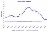
Cushing crude stocks sit less than 2 million bbls above operational floor amid global supply crisis
Cushing crude storage levels have plummeted in recent months. Inventories fell 11.3 million bbls to less than 25 million bbls between early April and early June, according to Wood Mackenzie.